Collaborative Filtering Part 2: Model-based Methods
by Yifei Zhou
1. Introduction
In the last section, I have outlined the memory-based collaborative filtering approaches. This method aims to compute and compare the similarity between users and items and select the nearest neighbours as the recommendation results. As I mentioned, the data sparsity issue seems critical as the database capacity is ample.
Model-based methods build an explicit or implicit model from the database. This type of method is widely used in collaborative filtering approaches. The model-based methods consist of different machine learning algorithms, such as classification, regression, clustering, deep learning, graph models, and matrix factorization.
In a real scenario, there are very few interactions between users and items in the database. The model-based methods aim to use these known interactions to predict potential interactions between users and items in unknown spaces.
2. Matrix Factorization
Matrix Factorization is one of the model-based collaborative-filtering methods. Basically, matrix factorization is a simple embedding approach. This type of method decompose a large sparse and high dimensional matrix into several lower dimensionality matrices.
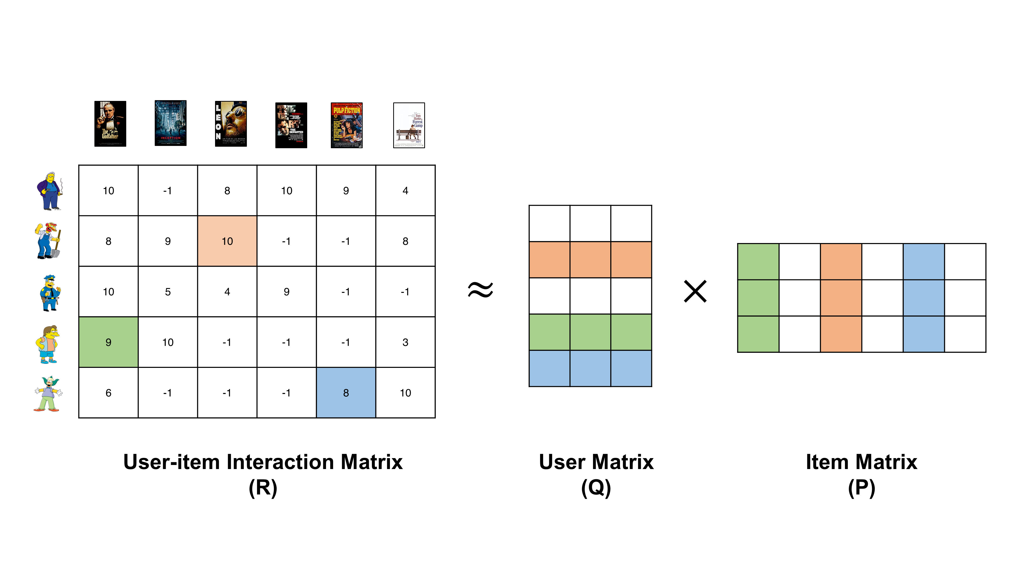
In a recommender system, the matrix factorization technique mainly refers to decompose a user-item matrix R into the product of two rectangular low-dimensionality dense matrices representing user-latent (P) and item-latent (Q) features, respectively.
 |
| Example of matrix factorizarion in user-item matrix |
2.1 PureSVD
Pure Singular Value Decomposition (PureSVD) is a classical application of Matrix Factorization. This method decomposes the user-item rating matrix into two orthogonal matrices representing user and item latent features and a diagonal matrix.
\[PureSVD(\textbf{R},f)=\textbf{P} \cdot \textbf{V} \cdot \textbf{Q}^{T}\]In the formula above, R is the user-item rating matrix, P and Q are user-latent and item-latent features, respectively. f is the dimensionality of the latent features.
2.2 EigenRec
EigenRec, argued by George Karypis, is an enhanced version of PureSVD, which supports customized scaling component for each item. Compared with PureSVD, this method requires one more parameter to control the item scaling component.
\[EigenRec(\textbf{R},d,f)=PureSVD(\textbf{R}Diag(\sqrt{\textbf{R}\textbf{R}^{T}})^{d-1},f)\]In the formula above, the item's scaling component is \(\textbf{R}\textbf{R}^{T}\), and the *d* is a parameter to control the factor. Interestingly, the EigenRec is same as the PureSVD when (d=1).
\[EigenRec(\textbf{R},d=1,f) = PureSVD(\textbf{R},f)\]3.Conclusion
PureSVD and EigenRec are the two most commonly used matrix factorization approaches. Both methods not only achieved better performance than the performance of neighbour-based methods but also reduced the computation and storage spaces. In addition, there are also some matrix factorization approaches, such as SVD++ and asymmetric SVD. These methods add different constraints on the users or items, but the outcomes are the same in producing two dense lower dimensionality matrices for users and items.
